Using Your Own Models

PeekingDuck offers pre-trained model nodes that can be used to tackle a wide variety of problems, but you may need to train your own model on a custom dataset sometimes. This tutorial will show you how to package your model into a custom model node, and use it with PeekingDuck. We will be tackling a manufacturing use case here - classifying images of steel castings into “defective” or “normal” classes.

Casting is a manufacturing process in which a material such as metal in liquid form is poured into a mold and allowed to solidify. The solidified result is also called a casting. Sometimes, defective castings are produced, and quality assurance departments are responsible for preventing defective pieces from being used downstream. As inspections are usually done manually, this adds a significant amount of time and cost, and thus there is an incentive to automate this process.

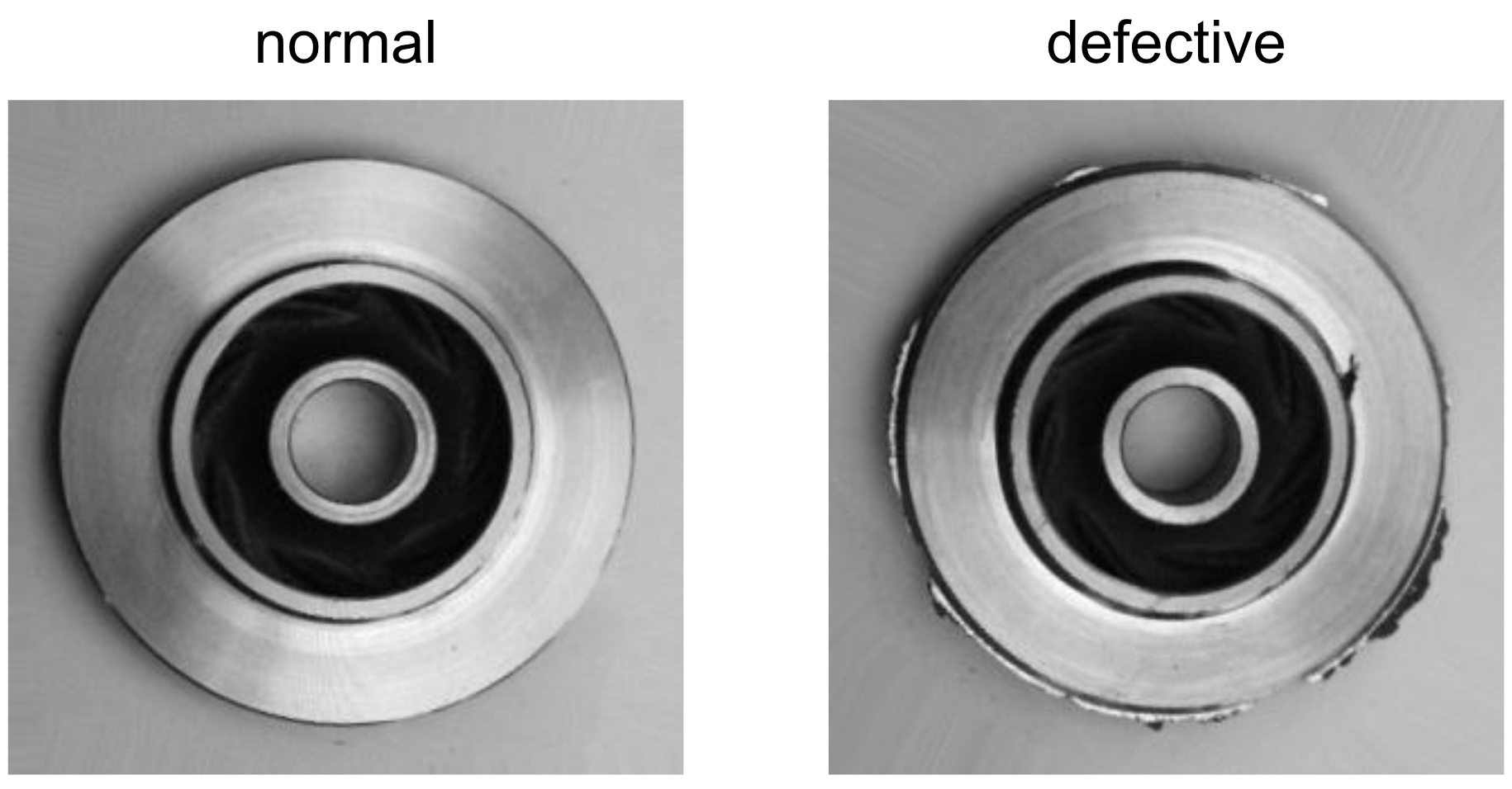
The images of castings used in this tutorial are the front faces of steel pump impellers. From the comparison below, it can be seen that the defective casting has a rough, uneven edges while the normal casting has smooth edges.

Normal Casting Compared to Defective Casting

Model Training

PeekingDuck is designed for model inference rather than model training. This optional section shows how a simple Convolutional Neural Network (CNN) model can be trained separately from the PeekingDuck framework. If you have already trained your own model, the following section describes how you can convert it to a custom model node, and use it within PeekingDuck for inference.

Setting Up

Install the following prerequisite for visualization.

> conda install matplotlib

Create the following project folder:

Terminal Session

[~user] > mkdir castings_project

[~user] > cd castings_project

Download the castings dataset and unzip the file to the castings_project folder.

Note

The castings dataset used in this example is modified from the original dataset from Kaggle.

You should have the following directory structure at this point:

castings_project/ ⠀
└── castings_data/ ⠀
      ├── inspection/ ⠀
      ├── train/ ⠀
      └── validation/ ⠀

Update Training Script

Create an empty train_classifier.py file within the castings_project folder, and update it with the following code:

train_classifier.py:

Show/Hide Code for train_classifier.py

"""
Script to train a classification model on images, save the model, and plot the training results

Adapted from: https://www.tensorflow.org/tutorials/images/classification
"""

import pathlib
from typing import List, Tuple

import matplotlib.pyplot as plt
import tensorflow as tf
from tensorflow.keras import layers
from tensorflow.keras.models import Sequential
from tensorflow.keras.layers.experimental.preprocessing import Rescaling

# setup global constants
DATA_DIR = "./castings_data"
WEIGHTS_DIR = "./weights"
RESULTS = "training_results.png"
EPOCHS = 10
BATCH_SIZE = 32
IMG_HEIGHT = 180
IMG_WIDTH = 180


def prepare_data() -> Tuple[tf.data.Dataset, tf.data.Dataset, List[str]]:
   """
   Generate training and validation datasets from a folder of images.

   Returns:
      train_ds (tf.data.Dataset): Training dataset.
      val_ds (tf.data.Dataset): Validation dataset.
      class_names (List[str]): Names of all classes to be classified.
   """

   train_dir = pathlib.Path(DATA_DIR, "train")
   validation_dir = pathlib.Path(DATA_DIR, "validation")

   train_ds = tf.keras.preprocessing.image_dataset_from_directory(
      train_dir,
      image_size=(IMG_HEIGHT, IMG_WIDTH),
      batch_size=BATCH_SIZE,
   )

   val_ds = tf.keras.preprocessing.image_dataset_from_directory(
      validation_dir,
      image_size=(IMG_HEIGHT, IMG_WIDTH),
      batch_size=BATCH_SIZE,
   )

   class_names = train_ds.class_names

   return train_ds, val_ds, class_names


def train_and_save_model(
   train_ds: tf.data.Dataset, val_ds: tf.data.Dataset, class_names: List[str]
) -> tf.keras.callbacks.History:
   """
   Train and save a classification model on the provided data.

   Args:
      train_ds (tf.data.Dataset): Training dataset.
      val_ds (tf.data.Dataset): Validation dataset.
      class_names (List[str]): Names of all classes to be classified.

   Returns:
      history (tf.keras.callbacks.History): A History object containing recorded events from
               model training.
   """

   num_classes = len(class_names)

   model = Sequential(
      [
            Rescaling(1.0 / 255, input_shape=(IMG_HEIGHT, IMG_WIDTH, 3)),
            layers.Conv2D(16, 3, padding="same", activation="relu"),
            layers.MaxPooling2D(),
            layers.Conv2D(32, 3, padding="same", activation="relu"),
            layers.MaxPooling2D(),
            layers.Conv2D(64, 3, padding="same", activation="relu"),
            layers.MaxPooling2D(),
            layers.Dropout(0.2),
            layers.Flatten(),
            layers.Dense(128, activation="relu"),
            layers.Dense(num_classes),
      ]
   )

   model.compile(
      optimizer="adam",
      loss=tf.keras.losses.SparseCategoricalCrossentropy(from_logits=True),
      metrics=["accuracy"],
   )

   print(model.summary())
   history = model.fit(train_ds, validation_data=val_ds, epochs=EPOCHS)
   model.save(WEIGHTS_DIR)

   return history


def plot_training_results(history: tf.keras.callbacks.History) -> None:
   """
   Plot training and validation accuracy and loss curves, and save the plot.

   Args:
      history (tf.keras.callbacks.History): A History object containing recorded events from
               model training.
   """
   acc = history.history["accuracy"]
   val_acc = history.history["val_accuracy"]
   loss = history.history["loss"]
   val_loss = history.history["val_loss"]
   epochs_range = range(EPOCHS)

   plt.figure(figsize=(16, 8))
   plt.subplot(1, 2, 1)
   plt.plot(epochs_range, acc, label="Training Accuracy")
   plt.plot(epochs_range, val_acc, label="Validation Accuracy")
   plt.legend(loc="lower right")
   plt.title("Training and Validation Accuracy")

   plt.subplot(1, 2, 2)
   plt.plot(epochs_range, loss, label="Training Loss")
   plt.plot(epochs_range, val_loss, label="Validation Loss")
   plt.legend(loc="upper right")
   plt.title("Training and Validation Loss")
   plt.savefig(RESULTS)


if __name__ == "__main__":
   train_ds, val_ds, class_names = prepare_data()
   history = train_and_save_model(train_ds, val_ds, class_names)
   plot_training_results(history)

Training the Model

Train the model by running the following command.

Terminal Session

[~user/castings_project] > python train_classifier.py

Note

For macOS Apple Silicon, the above code only works on macOS 12.x Monterey with the latest tensorflow-macos and tensorflow-metal versions. It will crash on macOS 11.x Big Sur due to bugs in the outdated tensorflow versions.

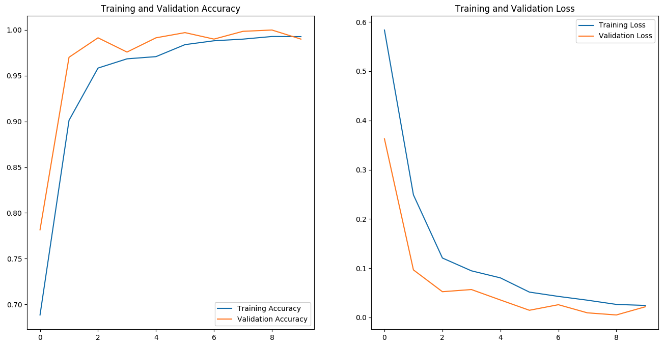
The model will be trained for 10 epochs, and when training is completed, a new weights folder and training_results.png will be created:

castings_project/ ⠀
├── train_classifier.py
├── training_results.png
├── castings_data/ ⠀
│     ├── inspection/ ⠀
│     ├── train/ ⠀
│     └── validation/ ⠀
└── weights/ ⠀
      ├── keras_metadata.pb
      ├── saved_model.pb
      ├── assets/ ⠀
      └── variables/ ⠀

The plots from training_results.png shown below indicate that the model has performed well on the validation dataset, and we are ready to create a custom model node from it.

Model Training Results

Using Your Trained Model with PeekingDuck

This section will show you how to convert your trained model into a custom PeekingDuck node, and give an example of how you can integrate this node in a PeekingDuck pipeline. It assumes that you are already familiar with the process of creating custom nodes, covered in the earlier custom node tutorial.

Converting to a Custom Model Node

First, let’s create a new PeekingDuck project within the existing castings_project folder.

Terminal Session

[~user/castings_project] > peekingduck init

Next, we’ll use the peekingduck create-node command to create a custom node:

Terminal Session

[~user/castings_project] > peekingduck create-node

Creating new custom node…

Enter node directory relative to ~user/castings_project [src/custom_nodes]: ⏎

Select node type (input, augment, model, draw, dabble, output): model

Enter node name [my_custom_node]: casting_classifier

Node directory: ~user/castings_project/src/custom_nodes

Node type: model

Node name: casting_classifier

Creating the following files:

Config file: ~user/castings_project/src/custom_nodes/configs/model/casting_classifier.yml

Script file: ~user/castings_project/src/custom_nodes/model/casting_classifier.py

Proceed? [Y/n]: ⏎

Created node!

The castings_project folder structure should now look like this:

castings_project/ ⠀
├── pipeline_config.yml
├── train_classifier.py
├── training_results.png
├── castings_data/ ⠀
│     ├── inspection/ ⠀
│     ├── train/ ⠀
│     └── validation/ ⠀
├── src/ ⠀
│     └── custom_nodes/ ⠀
│           ├── configs/ ⠀
│           │     └── model/ ⠀
│           │           └── casting_classifier.yml
│           └── model/ ⠀
│                 └── casting_classifier.py
└── weights/ ⠀
      ├── keras_metadata.pb
      ├── saved_model.pb
      ├── assets/ ⠀
      └── variables/ ⠀

castings_project now contains two files that we need to modify to implement our custom node.

1. src/custom_nodes/configs/model/casting_classifier.yml:

   casting_classifier.yml updated content:

   input: ["img"]
   output: ["pred_label", "pred_score"]
   
   weights_parent_dir: weights
   class_label_map: {0: "defective", 1: "normal"}
   

2. src/custom_nodes/model/casting_classifier.py:

   casting_classifier.py updated content:

   Show/Hide Code for casting_classifier.py

   """
   Casting classification model.
   """
   
   from typing import Any, Dict
   
   import cv2
   import numpy as np
   import tensorflow as tf
   
   from peekingduck.pipeline.nodes.node import AbstractNode
   
   IMG_HEIGHT = 180
   IMG_WIDTH = 180
   
   
   class Node(AbstractNode):
      """Initializes and uses a CNN to predict if an image frame shows a normal
      or defective casting.
      """
   
      def __init__(self, config: Dict[str, Any] = None, **kwargs: Any) -> None:
         super().__init__(config, node_path=__name__, **kwargs)
         self.model = tf.keras.models.load_model(self.weights_parent_dir)
   
      def run(self, inputs: Dict[str, Any]) -> Dict[str, Any]:
         """Reads the image input and returns the predicted class label and
         confidence score.
   
         Args:
               inputs (dict): Dictionary with key "img".
   
         Returns:
               outputs (dict): Dictionary with keys "pred_label" and "pred_score".
         """
         img = cv2.cvtColor(inputs["img"], cv2.COLOR_BGR2RGB)
         img = cv2.resize(img, (IMG_WIDTH, IMG_HEIGHT))
         img = np.expand_dims(img, axis=0)
         predictions = self.model.predict(img)
         score = tf.nn.softmax(predictions[0])
   
         return {
               "pred_label": self.class_label_map[np.argmax(score)],
               "pred_score": 100.0 * np.max(score),
         }
   

The custom node takes in the built-in PeekingDuck img data type, makes a prediction based on the image, and produces two custom data types: pred_label, the predicted label (“defective” or “normal”); and pred_score, which is the confidence score of the prediction.

Using the Classifier in a PeekingDuck Pipeline

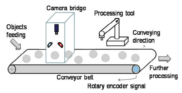
We’ll now pair this custom node with other PeekingDuck nodes to build a complete solution. Imagine an automated inspection system like the one shown below, where the castings are placed on a conveyor belt and a camera takes a picture of each casting and sends it to the PeekingDuck pipeline for prediction. A report showing the predicted result for each casting is produced, and the quality inspector can use it for further analysis.

Vision Based Inspection of Conveyed Objects (Source: ScienceDirect)

Edit the pipeline_config.yml file to use the input.visual node to read in the images, and the output.csv_writer node to produce the report. We will test our solution on the 10 casting images in castings_data/inspection, where each image’s filename is a unique casting ID such as 28_4137.jpeg.

pipeline_config.yml:

pipeline_config.yml updated content:

nodes:
- input.visual:
   source: castings_data/inspection
- custom_nodes.model.casting_classifier
- output.csv_writer:
   stats_to_track: ["filename", "pred_label", "pred_score"]
   file_path: casting_predictions.csv
   logging_interval: 0

Line 2 input.visual: tells PeekingDuck to load the images from castings_data/inspection.

Line 4 Calls the custom model node that you have just created.

Line 5 output.csv_writer: produces the report for the quality inspector in a CSV file castings_predictions_DDMMYY-hh-mm-ss.csv (time stamp appended to file_path). This node receives the filename data type from input.visual, the custom data types pred_label and pred_score from the custom model node, and writes them to the columns of the CSV file.

Run the above with the command peekingduck run.

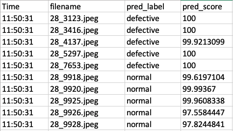
Open the created CSV file and you would see the following results. Half of the castings have been predicted as defective with high confidence scores. As the file name of each image is its unique casting ID, the quality inspector would be able to check the results with the actual castings if needed.

Casting Prediction Results

To visualize the predictions alongside the casting images, create an empty Python script named visualize_results.py, and update it with the following code:

visualize_results.py:

Show/Hide Code for visualize_results.py

"""
Script to visualize the prediction results alongside the casting images
"""

import csv

import cv2
import matplotlib.pyplot as plt

CSV_FILE = "casting_predictions_280422-11-50-30.csv"  # change file name accordingly
INSPECTION_IMGS_DIR = "castings_data/inspection/"
RESULTS_FILE = "inspection_results.png"

fig, axs = plt.subplots(2, 5, figsize=(50, 20))

with open(CSV_FILE) as csv_file:
   csv_reader = csv.reader(csv_file, delimiter=",")
   next(csv_reader, None)
   for i, row in enumerate(csv_reader):
      # csv columns follow this order: 'Time', 'filename', 'pred_label', 'pred_score'
      image_path = INSPECTION_IMGS_DIR + row[1]
      image_orig = cv2.imread(image_path)
      image_orig = cv2.cvtColor(image_orig, cv2.COLOR_BGR2RGB)

      row_idx = 0 if i < 5 else 1
      axs[row_idx][i % 5].imshow(image_orig)
      axs[row_idx][i % 5].set_title(row[1] + " - " + row[2], fontsize=35)
      axs[row_idx][i % 5].axis("off")

fig.savefig(RESULTS_FILE)

In Line 10, replace the name of CSV_FILE with the name of the CSV file produced on your system, as a timestamp would have been appended to the file name.

Run the following command to visualize the results.

Terminal Session

[~user/castings_project] > python visualize_results.py

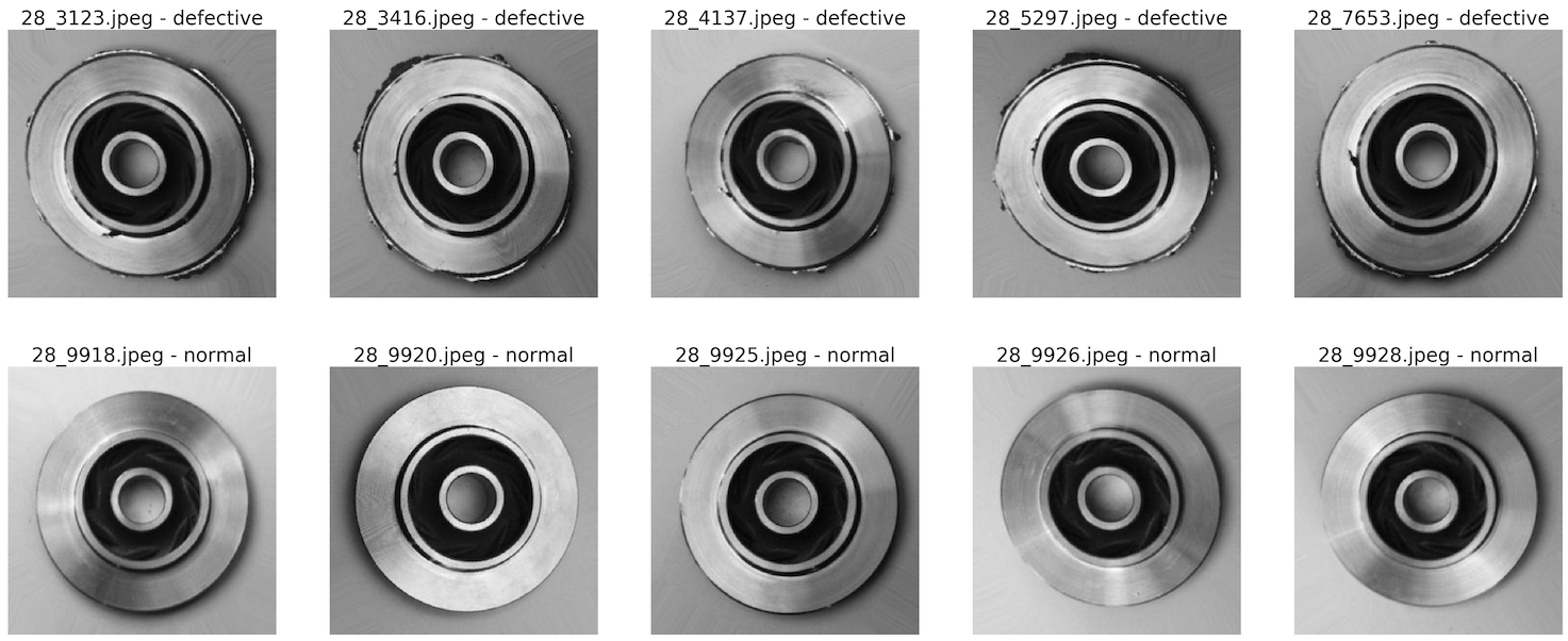
An inspection_results.png would be created, as shown below. The top row of castings are clearly defective, as they have rough, uneven edges, while the bottom row of castings look normal. Therefore, the prediction results are accurate for this batch of inspected castings. The quality inspector can provide feedback to the manufacturing team to further investigate the defective castings based on the casting IDs.

Casting Prediction Visualization

This concludes the guided example on using your own custom models.

Custom Object Detection Models

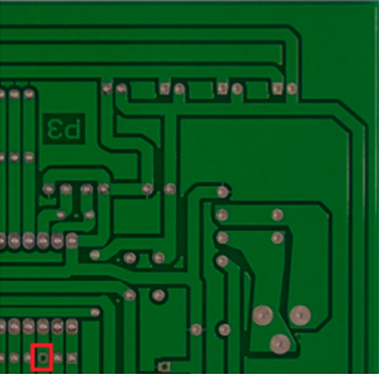
The previous example was centered on the task of image classification. Object detection is another common task in Computer Vision. PeekingDuck offers several pre-trained object detection model nodes which can detect up to 80 different types of objects, such as persons, cars, and dogs, just to name a few. For the complete list of detectable objects, refer to the Object Detection IDs page. Quite often, you may need to train a custom object detection model on your own dataset, such as defects on a printed circuit board (PCB) as shown below. This section discusses some important considerations for the object detection task, supplementing the guided example above.

Object Detection of Defects on PCB (Source: The Institution of Engineering and Technology)

PeekingDuck’s object detection model nodes conventionally receive the img data type, and produce the bboxes, bbox_labels, and bbox_scores data types. An example of this can be seen in the API documentation for a node such as model.efficientdet. We strongly recommend keeping to these data type conventions for your custom object detection node, ensuring that they adhere to the described format, e.g. img is in BGR format, and bboxes is a NumPy array of a certain shape.

This allows you to leverage on PeekingDuck’s ecosystem of existing nodes. For example, by ensuring that your custom model node receives img in the correct format, you are able to use PeekingDuck’s input.visual node, which can read from multiple visual sources such as a folder of images or videos, an online cloud source, or a CCTV/webcam live feed. By ensuring that your custom model node produces bboxes and bbox_labels in the correct format, you are able to use PeekingDuck’s draw.bbox node to draw bounding boxes and associated labels around the detected objects.

By doing so, you would have saved a significant amount of development time, and can focus more on developing and finetuning your custom object detection model. This was just a simple example, and you can find out more about PeekingDuck’s nodes from our API Documentation, and PeekingDuck’s built-in data types from our Glossary.